Cubic function
In mathematics, a cubic function is a function of the form
where a is nonzero; or in other words, a polynomial of degree three. The derivative of a cubic function is a quadratic function. The integral of a cubic function is a quartic function.
Setting ƒ(x) = 0 produces a cubic equation of the form:
Usually, the coefficients a, b,c, d are real numbers. However, most of the theory is also valid if they belong to a field of characteristic other than 2 or 3. To solve a cubic equation is to find the roots (zeros) of a cubic function. There are various ways to solve a cubic equation. The roots of a cubic, like those of a quadratic or quartic (fourth degree) function but no higher degree function, can always be found algebraically (as a formula involving simple functions like the square root and cube root functions). The roots can also be found trigonometrically. Alternatively, one can find a numerical approximation of the roots in the field of the real or complex numbers. This may be obtained by any root-finding algorithm, like Newton's method.
Solving cubic equations is a necessary part of solving the general quartic equation, since solving the latter requires solving its resolvent cubic equation.
Contents
|
History
Cubic equations were known to ancient Greek mathematician Diophantus;[1] even earlier to ancient Babylonians who were able to solve certain cubic equations;[2] and also to the ancient Egyptians. Doubling the cube is the simplest and oldest studied cubic equation, and one which the ancient Egyptians considered to be impossible.[3] Hippocrates reduced this problem to that of finding two mean proportionals between one line and another of twice its length, but could not solve this with a compass and straightedge construction,[4] a task which is now known to be impossible. Hippocrates, Menaechmus and Archimedes are believed to have come close to solving the problem of doubling the cube using intersecting conic sections,[4] though historians such as Reviel Netz dispute whether the Greeks were thinking about cubic equations or just problems that can lead to cubic equations. Some others like T. L. Heath, who translated all Archimedes' works, disagree, putting forward evidence that Archimedes really solved cubic equations using intersections of two cones, but also discussed the conditions where the roots are 0, 1 or 2.[5]
In the 7th century, the Tang dynasty astronomer mathematician Wang Xiaotong in his mathematical treatise titled Jigu Suanjing systematically established and solved 25 cubic equations of the form  , 23 of them with
  , and two of them with
  .[6]
.[6]
In the 11th century, the Persian poet-mathematician, Omar Khayyám (1048–1131), made significant progress in the theory of cubic equations. In an early paper he wrote regarding cubic equations, he discovered that a cubic equation can have more than one solution and stated that it cannot be solved using compass and straightedge constructions. He also found a geometric solution, which could be used to get a numerical answer by consulting trigonometric tables[7] [8]. In his later work, the Treatise on Demonstration of Problems of Algebra, he wrote a complete classification of cubic equations with general geometric solutions found by means of intersecting conic sections.[9][10]
In the 12th century, the Indian mathematician Bhaskara II attempted the solution of cubic equations without general success. However, he gave one example of a cubic equation:[11]
In the 12th century, another Persian mathematician, Sharaf al-Dīn al-Tūsī (1135–1213), wrote the Al-Mu'adalat (Treatise on Equations), which dealt with eight types of cubic equations with positive solutions and five types of cubic equations which may not have positive solutions. He used what would later be known as the "Ruffini-Horner method" to numerically approximate the root of a cubic equation. He also developed the concepts of a derivative function and the maxima and minima of curves in order to solve cubic equations which may not have positive solutions.[12] He understood the importance of the discriminant of the cubic equation to find algebraic solutions to certain types of cubic equations.[13]
Leonardo de Pisa, also known as Fibonacci (1170–1250), was able to find the positive solution to the cubic equation x3+2x2+10x = 20, using the Babylonian numerals. He gave the result as 1,22,7,42,33,4,40 which is equivalent to: 1+22/60+7/602+42/603+33/604+4/605+40/606.[14]
In the early 16th century, the Italian mathematician Scipione del Ferro (1465–1526) found a method for solving a class of cubic equations, namely those of the form x3 + mx = n. In fact, all cubic equations can be reduced to this form if we allow m and n to be negative, but negative numbers were not known to him at that time. Del Ferro kept his achievement secret until just before his death, when he told his student Antonio Fiore about it.
In 1530, Niccolò Tartaglia (1500–1557) received two problems in cubic equations from Zuanne da Coi and announced that he could solve them. He was soon challenged by Fiore, which led to a famous contest between the two. Each contestant had to put up a certain amount of money and to propose a number of problems for his rival to solve. Whoever solved more problems within 30 days would get all the money. Tartaglia received questions in the form x3 + mx = n, for which he had worked out a general method. Fiore received questions in the form x3 + mx2 = n, which proved to be too difficult for him to solve, and Tartaglia won the contest.
Later, Tartaglia was persuaded by Gerolamo Cardano (1501–1576) to reveal his secret for solving cubic equations. In 1539, Tartaglia did so only on the condition that Cardano would never reveal it and that if he did reveal a book about cubics, that he would give Tartaglia time to publish. Some years later, Cardano learned about Ferro's prior work and published Ferro's method in his book Ars Magna in 1545, meaning Cardano gave Tartaglia 6 years to publish his results (with credit given to Tartaglia for an independent solution). Cardano's promise with Tartaglia stated that he not publish Tartaglia's work, and Cardano felt he was publishing del Ferro's, so as to get around the promise. Nevertheless, this led to a challenge to Cardano by Tartaglia, which Cardano denied. The challenge was eventually accepted by Cardano's student Lodovico Ferrari (1522–1565). Ferrari did better than Tartaglia in the competition, and Tartaglia lost both his prestige and income.[15]
Cardano noticed that Tartaglia's method sometimes required him to extract the square root of a negative number. He even included a calculation with these complex numbers in Ars Magna, but he did not really understand it. Rafael Bombelli studied this issue in detail and is therefore often considered as the discoverer of complex numbers.
François Viète (1540–1603) independently derived the trigonometric solution for the cubic with three real roots, and René Descartes (1596–1650) extended the work of Viète.[16]
Derivative
Through the quadratic formula the roots of the derivative f′(x) = 3ax2 + 2bx + c are given by

and provide the critical points where the slope of the cubic function is zero. If b2 − 3ac > 0, then the cubic function has a local maximum and a local minimum. If b2 − 3ac = 0, then the cubic's inflection point is the only critical point. If b2 − 3ac < 0, then there are no critical points. In the cases where b2 − 3ac ≤ 0, the cubic function is strictly monotonic.
Roots of a cubic function
The general cubic equation has the form

with 
This section describes how the roots of such an equation may be computed. The coefficients a, b, c, d are generally assumed to be real numbers, but most of the results apply when they belong to any field of characteristic not 2 or 3.
The nature of the roots
Every cubic equation (1) with real coefficients has at least one solution x among the real numbers; this is a consequence of the intermediate value theorem. We can distinguish several possible cases using the discriminant,

The following cases need to be considered: [17]
- If Δ > 0, then the equation has three distinct real roots.
- If Δ = 0, then the equation has a multiple root and all its roots are real.
- If Δ < 0, then the equation has one real root and two nonreal complex conjugate roots.
General formula of roots
For the general cubic equation (1) with real coefficients, the general formula for the roots, in terms of the coefficients, is as follows. Note that the expression under the square root sign in what follows is  , where
  is the above-mentioned discriminant.
![\begin{align}
x_1 =
&-\frac{b}{3 a}\\
&-\frac{1}{3 a} \sqrt[3]{\tfrac12\left[2 b^3-9 a b c%2B27 a^2 d%2B\sqrt{\left(2 b^3-9 a b c%2B27 a^2 d\right)^2-4 \left(b^2-3 a c\right)^3}\right]}\\
&-\frac{1}{3 a} \sqrt[3]{\tfrac12\left[2 b^3-9 a b c%2B27 a^2 d-\sqrt{\left(2 b^3-9 a b c%2B27 a^2 d\right)^2-4 \left(b^2-3 a c\right)^3}\right]}\\
x_2 =
&-\frac{b}{3 a}\\
&%2B\frac{1%2Bi \sqrt{3}}{6 a} \sqrt[3]{\tfrac12\left[2 b^3-9 a b c%2B27 a^2 d%2B\sqrt{\left(2 b^3-9 a b c%2B27 a^2 d\right)^2-4 \left(b^2-3 a c\right)^3}\right]}\\
&%2B\frac{1-i \sqrt{3}}{6 a} \sqrt[3]{\tfrac12\left[2 b^3-9 a b c%2B27 a^2 d-\sqrt{\left(2 b^3-9 a b c%2B27 a^2 d\right)^2-4 \left(b^2-3 a c\right)^3}\right]}\\
x_3 =
&-\frac{b}{3 a}\\
&%2B\frac{1-i \sqrt{3}}{6 a} \sqrt[3]{\tfrac12\left[2 b^3-9 a b c%2B27 a^2 d%2B\sqrt{\left(2 b^3-9 a b c%2B27 a^2 d\right)^2-4 \left(b^2-3 a c\right)^3}\right]}\\
&%2B\frac{1%2Bi \sqrt{3}}{6 a} \sqrt[3]{\tfrac12\left[2 b^3-9 a b c%2B27 a^2 d-\sqrt{\left(2 b^3-9 a b c%2B27 a^2 d\right)^2-4 \left(b^2-3 a c\right)^3}\right]}
\end{align}](/2012-wikipedia_en_all_nopic_01_2012/I/7f19af779a9bea4db300039405693001.png)
However, this formula is applicable without further explanation only when the operand of the square root is non-negative and a,b,c,d are real coefficients. When this operand is real and non-negative, the square root refers to the principal (positive) square root and the cube roots in the formula are to be interpreted as the real ones. Otherwise, there is no real square root and one can arbitrarily choose one of the imaginary square roots (the same one in both parts of the solution for each xi). For extracting the complex cube roots of the resulting complex expression, we have also to choose among three cube roots in each part of each solution, giving nine possible combinations of one of three cube roots for the first part of the expression and one of three for the second. The correct combination is such that the two cube roots chosen for the two terms in a given solution expression are complex conjugates of each other (whereby the two imaginary terms in each solution cancel out).
Another way of writing the solution may be obtained by noting that the proof of above formula shows that the product of the two cube roots is rational. This gives the following formula in which  or
or ![\sqrt[3]{ }](/2012-wikipedia_en_all_nopic_01_2012/I/9bbd095bafd3ae229d6baa25f34ebe84.png) stands for any choice of the square or cube root, if
stands for any choice of the square or cube root, if 
![\begin{align}
Q = &\sqrt{(2 b^3-9 a b c%2B27 a^2 d)^2-4 (b^2-3 a c)^3}\\
C = &\sqrt[3]{\tfrac12 (Q %2B 2 b^3-9 a b c%2B27 a^2 d)}\\
x_1 = &-\frac{b}{3 a}-\frac{C}{3 a}-\frac{b^2-3 a c}{3 a C}\\
x_2 = &-\frac{b}{3 a}%2B\frac{C(1%2Bi \sqrt{3})}{6 a} %2B\frac{(1-i \sqrt{3}) (b^2-3 a c)}{6 a C}\\
x_3 = &-\frac{b}{3 a}%2B\frac{C(1-i \sqrt{3})}{6 a} %2B\frac{(1%2Bi \sqrt{3}) (b^2-3 a c)}{6 a C}
\end{align}](/2012-wikipedia_en_all_nopic_01_2012/I/348ffa4b63eb0ddd0c4391c9605e6865.png)
If  and
and  , the sign of
  has to be chosen to have
  .
.
If  and , the three roots are equal:
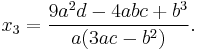
If  and
and  , the above expression for the roots is correct but misleading, hiding the fact that no radical is needed to represent the roots. In fact, in this case, there is a double root,
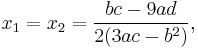
and a simple root
The next sections describe how these formulas may be obtained.
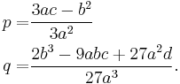
Reduction to a monic trinomial
Dividing Equation (1) by  and substituting
  by
by  (the Tschirnhaus transformation) we get the equation
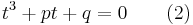
where
Any formula for the roots of Equation (2) may be transformed into a formula for the roots of Equation (1) by substituting the above values for  and
and  and using the relation
  .
.
Therefore, only Equation (2) is considered in the following.
Cardano's method
The solutions can be found with the following method due to Scipione del Ferro and Tartaglia, published by Gerolamo Cardano in 1545.[18]
We first apply preceding reduction, giving the so-called depressed cubic
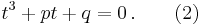
We introduce two variables u and v linked by the condition

and substitute this in the depressed cubic (2), giving
 .
.
At this point Cardano imposed a second condition for the variables u and v:
 .
.
As the first parenthesis vanishes in (3), we get 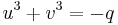 and
and 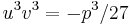 . Thus
  and
and  are the two roots of the equation
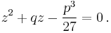
At this point, Cardano, who did not know complex numbers, supposed that the roots of this equation were real, that is that 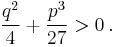
Solving this equation and using the fact that  and
and  may be exchanged, we find
 and
and 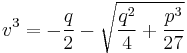 .
.
As these expressions are real, their cube roots are well defined and, like Cardano, we get
![t_1=u%2Bv=\sqrt[3]{-{q\over 2}%2B \sqrt{{q^{2}\over 4}%2B{p^{3}\over 27}}} %2B\sqrt[3]{-{q\over 2}- \sqrt{{q^{2}\over 4}%2B{p^{3}\over 27}}}](/2012-wikipedia_en_all_nopic_01_2012/I/621f6bb67577ad721951719e7b662f0a.png)
The two complex roots are obtained by considering the complex cubic roots; the fact  is real implies that they are obtained by multiplying one of the above cubic roots by
  and the other by
  .
.
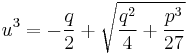
If  is not necessarily positive, we have to choose a cube root of . As there is no direct way to choose the corresponding cube root of , one has to use the relation
  , which gives
![u=\sqrt[3]{-{q\over 2}- \sqrt{{q^{2}\over 4}%2B{p^{3}\over 27}}} \qquad (4)](/2012-wikipedia_en_all_nopic_01_2012/I/e77e15ea1779eb73fc57728535517c0b.png)
and
Note that the sign of the square root does not affect the resulting  , because changing it amounts to exchanging and . We have chosen the minus sign to have
  when
when  and
and  , in order to avoid a division by zero. With this choice, the above expression for always works, except when
  , where the second term becomes 0/0. In this case there is a triple root
  .
.
Note also that in several cases the solutions are expressed with fewer square or cube roots
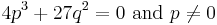
- If then we have the triple real root
- If and then
- and the three roots are the three cube roots of
 .
. - If
 and then
- in which case the three roots are
- where
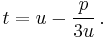
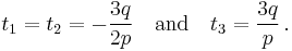
- Finally if
 , there is a double root and a simple root which may be expressed rationally in term of
  , but this expression may not be immediately deduced from the general expression of the roots:

![u=-\sqrt[3]{q} \text{ and } v = 0](/2012-wikipedia_en_all_nopic_01_2012/I/21ce5e3b05a268ece1049819132e57ae.png)

To pass from these roots of in Equation (2) to the general formulas for roots of in Equation (1), subtract  and replace and by their expressions in terms of
  .
.
Lagrange's method
In his paper Réflexions sur la résolution algébrique des équations ("Thoughts on the algebraic solving of equations"), Joseph Louis Lagrange introduced a new method to solve equations of low degree.
This method works well for cubic and quartic equations, but Lagrange did not succeed in applying it to a quintic equation, because it requires solving a resolvent polynomial of degree at least six.[19][20][21] This is explained by the Abel–Ruffini theorem, which proves that such polynomials cannot be solved by radicals. Nevertheless the modern methods for solving solvable quintic equations are mainly based on Lagrange's method.[21]
In the case of cubic equations, Lagrange's method gives the same solution as Cardano's, but avoids its seemingly magical aspect (Why did Cardano choose these auxiliary variables?). Moreover, it may also be applied directly to the general cubic equation (1) without using the reduction to the trinomial equation (2). Nevertheless the computation is much easier with this reduced equation.
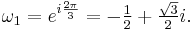
Suppose that x0, x1 and x2 are the roots of equation (1) or (2), and define  , so that ζ is a primitive third root of unity which satisfies the relation
  . We now set
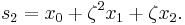
This is the discrete Fourier transform of the roots: observe that while the coefficients of the polynomial are symmetric in the roots, in this formula an order has been chosen on the roots, so these are not symmetric in the roots. The roots may then be recovered from the three si by inverting the above linear transformation via the inverse discrete Fourier transform, giving
The polynomial  is an elementary symmetric polynomial and is thus equal to
  in case of Equation (1) and to zero in case of Equation (2), so we only need to seek values for the other two.
The polynomials  and
and  are not symmetric functions of the roots: is invariant, while the two non-trivial cyclic permutations of the roots send to
  and to
  , or to
  and to
  (depending on which permutation), while transposing
  and
and  switches and ; other transpositions switch these roots and multiply them by a power of
Thus,  ,
,  and
and  are left invariant by the cyclic permutations of the roots, which multiply them by
  . Also and
  are left invariant by the transposition of and which exchanges and . As the permutation group
  of the roots is generated by these permutations, it follows that and are symmetric functions of the roots and may thus be written as polynomials in the elementary symmetric polynomials and thus as rational functions of the coefficients of the equation. Let
  and
and  in these expressions, which will be explicitly computed below.
We have that and are the two roots of the quadratic equation
Thus the resolution of the equation may be finished exactly as described for Cardano's method, with and in place of and .
Computation of A and B
Setting  ,
,  and
and  , the elementary symmetric polynomials, we have, using that :

The expression for is the same with  and
and  exchanged. Thus, using
  we get

and a straightforward computation gives

Similarly we have

When solving Equation (1) we have
 ,
,  and
and 
With Equation (2), we have  ,
,  and
and  and thus:
 and
and  .
.
Note that with Equation (2), we have  and
and  , while in Cardano's method we have set
  and
and  Thus we have, up to the exchange of and :
 and
and  .
.
In other words, in this case, Cardano's and Lagrange's method compute exactly the same things, up to a factor of three in the auxiliary variables, the main difference being that Lagrange's method explains why these auxiliary variables appear in the problem.
Trigonometric (and hyperbolic) method
When a cubic equation has three real roots, the formulas expressing these roots in terms of radicals involve complex numbers. It has been proved that when none of the three real roots is rational—the casus irreducibilis— one cannot express the roots in terms of real radicals. Nevertheless, purely real expressions of the solutions may be obtained using hypergeometric functions,[22] or more elementarily in terms of trigonometric functions, specifically in terms of the cosine and arccosine functions.
The formulas which follow, due to François Viète,[16] are true in general (except when p = 0), are purely real when the equation has three real roots, but involve complex cosines and arccosines when there is only one real root.
Starting from Equation (2), 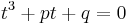 , let us set
 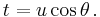 The idea is to choose to make Equation (2) coincide with the identity

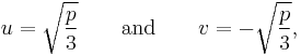
In fact, choosing  and dividing Equation (2) by
  we get
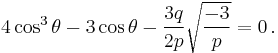
Combining with the above identity, we get
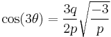
and thus the roots are[23]

This formula involves only real terms if  and the argument of the arccosine is between −1 and 1. The last condition is equivalent to
  which implies also . Thus the above formula for the roots involves only real terms if and only if the three roots are real.
Denoting by  the above value of t0, and using the inequality
  for a real number u such that
  the three roots may also be expressed as

If the three roots are real, we have
All these formulas may be straightforwardly transformed into formulas for the roots of the general cubic equation (1), using the back substitution described in Section Reduction to a monic trinomial.
When there is only one real root (and p ≠ 0), it may be similarly represented using hyperbolic functions, as[24][25]

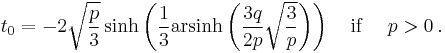
If p ≠ 0 and the inequalities on the right are not satisfied the formulas remain valid but involve complex quantities.
When  , the above values of
  are sometimes called the Chebyshev cube root.[26] More precisely, the values involving cosines and hyperbolic cosines define, when
  , the same analytic function denoted
  , which is the proper Chebyshev cube root. The value involving hyperbolic sines is similarly denoted
  when
when  .
.
Factorization
If the cubic equation 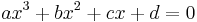 with integer coefficients has a rational real root, it can be found using the rational root test: If the root is r = m / n fully reduced, then m is a factor of d and n is a factor of a, so all possible combinations of values for m and n can be checked for whether they satisfy the cubic equation. This is particularly useful when there are three real roots, since in this case as indicated previously the algebraic solution unhelpfully expresses the real roots in terms of complex entities.
If r is any root of the cubic, then we may factor out (x–r ) using polynomial long division to obtain

Hence if we know one root we can find the other two by using the quadratic formula to solve the quadratic  , giving
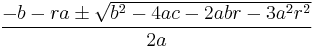
for the other two roots.
If there are three real roots and none of them is rational, we have the so-called casus irreducibilis in which the cubic cannot be factored into the product of a linear polynomial and a quadratic polynomial each with real coefficients.
Geometric interpretation of the roots
Three real roots
Viète's trigonometric expression of the roots in the three-real-roots case lends itself to a geometric interpretation in terms of a circle.[16][27] When the cubic is written as above as , as shown above the solution can be expressed as
Here 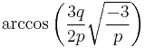 is an angle in the unit circle; taking
  of that angle corresponds to taking a cube root of a complex number; adding
  for k = 1, 2 finds the other cube roots; and multiplying the cosines of these resulting angles by
  corrects for scale.
One real and two complex roots
In the Cartesian plane
If a cubic is plotted in the Cartesian plane, the real root can be seen graphically as the horizontal intercept of the curve. But further,[28][29][30] if the complex conjugate roots are written as g+hi, then g is the abscissa (the positive or negative horizontal distance from the origin) of the tangency point of a line that is tangent to the cubic curve and intersects the horizontal axis at the same place as does the cubic curve; and |h| is the square root of the tangent of the angle between this line and the horizontal axis.
In the complex plane
With one real and two complex roots, the three roots can be represented as points in the complex plane, as can the two roots of the cubic's derivative. There is an interesting geometrical relationship among all these roots.
The points in the complex plane representing the three roots serve as the vertices of an isosceles triangle. (The triangle is isosceles because one root is on the horizontal (real) axis and the other two roots, being complex conjugates, appear symmetrically above and below the real axis.) Marden's Theorem says that the points representing the roots of the derivative of the cubic are the foci of the Steiner inellipse of the triangle—the unique ellipse that is tangent to the triangle at the midpoints of its sides. If the angle at the vertex on the real axis is less than  then the major axis of the ellipse lies on the real axis, as do its foci and hence the roots of the derivative. If that angle is greater than , the major axis is vertical and its foci, the roots of the derivative, are complex. And if that angle is , the triangle is equilateral, the Steiner inellipse is simply the triangle's incircle, its foci coincide with each other at the incenter, which lies on the real axis, and hence the derivative has duplicate real roots.
Omar Khayyám's solution
As shown in this graph, to solve the third-degree equationOmar Khayyám constructed the parabola
a circle with diameter
and a vertical line through an intersection point. The solution is given by the length of the horizontal line segment from the origin to the intersection of the vertical line and the x-axis.
See also
- Linear equation
- Quadratic equation
- Quartic equation
- Quintic equation
- Polynomial
- Newton's method
- Spline (mathematics)
Notes
- ^ Van de Waerden, Geometry and Algebra of Ancient Civilizations, chapter 4, Zurich 1983 ISBN 0387121595
- ^ British Museum BM 85200
- ^ Guilbeau (1930, p. 8) states, "The Egyptians considered the solution impossible, but the Greeks came nearer to a solution."
- ^ a b Guilbeau (1930, pp. 8–9)
- ^ The works of Archimedes, translation by T. L. Heath
- ^ Mikami, Yoshio (1974) [1913], "Chapter 8 Wang Hsiao-Tung and Cubic Equations", The Development of Mathematics in China and Japan (2nd ed.), New York: Chelsea Publishing Co., pp. 53–56, ISBN 978-0828401494
- ^ A paper of Omar Khayyam, Scripta Math. 26 (1963), pages 323-337
- ^ O'Connor, John J.; Robertson, Edmund F., "Omar Khayyam", MacTutor History of Mathematics archive, University of St Andrews, http://www-history.mcs.st-andrews.ac.uk/Biographies/Khayyam.html.
- ^ J. J. O'Connor and E. F. Robertson (1999), Omar Khayyam, MacTutor History of Mathematics archive, states, "Khayyam himself seems to have been the first to conceive a general theory of cubic equations."
- ^ Guilbeau (1930, p. 9) states, "Omar Al Hay of Chorassan, about 1079 AD did most to elevate to a method the solution of the algebraic equations by intersecting conics."
- ^ Datta and Singh, History of Hindu Mathematics, p76,Equation of Higher Degree; Bharattya Kala Prakashan, Delhi, India 2004 ISBN 81-86050-86-8
- ^ O'Connor, John J.; Robertson, Edmund F., "Sharaf al-Din al-Muzaffar al-Tusi", MacTutor History of Mathematics archive, University of St Andrews, http://www-history.mcs.st-andrews.ac.uk/Biographies/Al-Tusi_Sharaf.html.
- ^ J. L. Berggren (1990), "Innovation and Tradition in Sharaf al-Din al-Tusi's Muadalat", Journal of the American Oriental Society 110 (2): 304–9
- ^ "The life and numbers of Fibonacci" [1], Plus Magazine
- ^ Katz, Victor. A History of Mathematics. pp. 220. Boston: Addison Wesley, 2004.
- ^ a b c Nickalls, R. W. D., "Viète, Descartes and the cubic equation," Mathematical Gazette 90, July 2006, 203–208.
- ^ Irving, Ronald S. (2004), Integers, polynomials, and rings, Springer-Verlag New York, Inc., ISBN 0-387-40397-3, http://books.google.com/?id=B4k6ltaxm5YC, Chapter 10 ex 10.14.4 and 10.17.4, pp. 154–156
- ^ Jacobson (2009), p. 210.
- ^ Prasolov, Viktor; Solovyev, Yuri (1997), Elliptic functions and elliptic integrals, AMS Bookstore, ISBN 978 0 82180587 9, http://books.google.com/?id=fcp9IiZd3tQC, §6.2, p. 134
- ^ Kline, Morris (1990), Mathematical Thought from Ancient to Modern Times, Oxford University Press US, ISBN 978 0 19506136 9, http://books.google.com/?id=aO-v3gvY-I8C, Algebra in the Eighteenth Century: The Theory of Equations
- ^ a b Daniel Lazard, "Solving quintics in radicals", in Olav Arnfinn Laudal, Ragni Piene, The Legacy of Niels Henrik Abel, pp. 207–225, Berlin, 2004,. ISBN 3-5404-3826-2
- ^ Zucker, I. J., "The cubic equation — a new look at the irreducible case", Mathematical Gazette 92, July 2008, 264–268.
- ^ Shelbey, Samuel (1975), CRC Standard Mathematical Tables, CRC Press, ISBN 0 87819 622 6
- ^ These are Formulas (80) and (83) of Weisstein, Eric W. 'Cubic Formula'. From MathWorld—A Wolfram Web Resource. http://mathworld.wolfram.com/CubicFormula.html, rewritten for having a coherent notation.
- ^ Holmes, G. C., "The use of hyperbolic cosines in solving cubic polynomials", Mathematical Gazette 86. November 2002, 473–477.
- ^ Abramowitz, Milton; Stegun, Irene A., eds. Handbook of Mathematical Functions with Formulas, Graphs, and Mathematical Tables, Dover (1965), chap. 22 p. 773
- ^ Nickalls, R. W. D. (November 1993), "A new approach to solving the cubic: Cardan's solution revealed", The Mathematical Gazette 77 (480): 354–359, doi:10.2307/3619777, ISSN 0025-5572, JSTOR 3619777, http://www.nickalls.org/dick/papers/maths/cubic1993.pdf See esp. Fig. 2.
- ^ Henriquez, G., "The graphical interpretation of the complex roots of cubic equations," American Mathematical Monthly 42, June–July 1935, 383–384.
- ^ Barr, C. F., American Mathematical Monthly 25, 1918, p. 268
- ^ Barr, C. F., Annals of Mathematics 19, 1917, p. 157.
References
- Anglin, W. S.; Lambek, Joachim (1995), "Mathematics in the Renaissance", The Heritage of Thales, Springers, pp. 125–131, ISBN 978-0387945446, http://books.google.com/?id=mZfXHRgJpmQC&pg=PA125&lpg=PA125&dq=%22mathematics+in+the+renaissance%22+heritage+thales&q Ch. 24.
- Guilbeau, Lucye (1930), "The History of the Solution of the Cubic Equation", Mathematics News Letter 5 (4): 8–12, doi:10.2307/3027812, JSTOR 3027812
- Jacobson, Nathan (2009), Basic algebra, 1 (2nd ed.), Dover, ISBN 978-0-486-47189-1
- Dunnett, R., "Newton–Raphson and the cubic," Mathematical Gazette 78, November 1994, 347–348.
- Dence, T., "Cubics, chaos and Newton's method," Mathematical Gazette 81, November 1997, 403–408.
- Mitchell, D. W., "Solving cubics by solving triangles," Mathematical Gazette 91, November 2007, 514–516.
- Press, WH; Teukolsky, SA; Vetterling, WT; Flannery, BP (2007), "Section 5.6 Quadratic and Cubic Equations", Numerical Recipes: The Art of Scientific Computing (3rd ed.), New York: Cambridge University Press, ISBN 978-0-521-88068-8, http://apps.nrbook.com/empanel/index.html?pg=227
- Zucker, I. J., "The cubic equation—A new look at the irreducible case," Mathematical Gazette 92, July 2008, 264–268.
- Rechtschaffen, E., "Real roots of cubics: Explicit formula for quasi-solutions," Mathematical Gazette 92, July 2008, 268–276.
- Mitchell, D. W., "Powers of
 as roots of cubics," Mathematical Gazette 93, November 2009.
External links
- Solving a Cubic by means of Moebius transforms
- Interesting derivation of trigonometric cubic solution with 3 real roots
- Calculator for solving Cubics (also solves Quartics and Quadratics)
- Tartaglia's work (and poetry) on the solution of the Cubic Equation at Convergence
- Cubic Equation Solver.
- Quadratic, cubic and quartic equations on MacTutor archive.
- Cubic Formula on PlanetMath
- Cardano solution calculator as java applet at some local site. Only takes natural coefficients.
- Graphic explorer for cubic functions With interactive animation, slider controls for coefficients
- On Solution of Cubic Equations at Holistic Numerical Methods Institute
- Dave Auckly, Solving the quartic with a pencil American Math Monthly 114:1 (2007) 29—39
- "Cubic Equation" by Eric W. Weisstein, The Wolfram Demonstrations Project, 2007.
- The affine equivalence of cubic polynomials at Dynamic Geometry Sketches
|
||||||||